32 混合效应模型
\[ \def\bm#1{{\boldsymbol #1}} \]
混合效应模型在心理学、生态学、计量经济学和空间统计学等领域应用十分广泛。混合效应模型内容非常多,非常复杂,因此,本章仅对常见的四种类型提供入门级的实战内容。从频率派和贝叶斯派两个角度介绍模型结构及说明、R 代码或 Stan 代码实现及输出结果解释。
本章用到 4 个数据集,其中 sleepstudy 和 cbpp 均来自 lme4 包,分别用于介绍线性混合效应模型和广义线性混合效应模型,Loblolly 来自 datasets 包,用于介绍非线性混合效应模型,最后,朗格拉普岛核辐射数据数据集用于介绍广义可加混合效应模型。
32.1 线性混合效应模型
32.1.1 频率派
32.1.1.1 nlme
#> 'data.frame':    180 obs. of  3 variables:
#>  $ Reaction: num  250 259 251 321 357 ...
#>  $ Days    : num  0 1 2 3 4 5 6 7 8 9 ...
#> $ Subject : Factor w/ 18 levels "308","309","310",..: 1 1 1 1 1 1 1 1 1 1 ...library(ggplot2)
ggplot(data = sleepstudy, aes(x = Days, y = Reaction, group = Subject)) +
geom_line() +
scale_x_continuous(n.breaks = 6) +
theme_bw()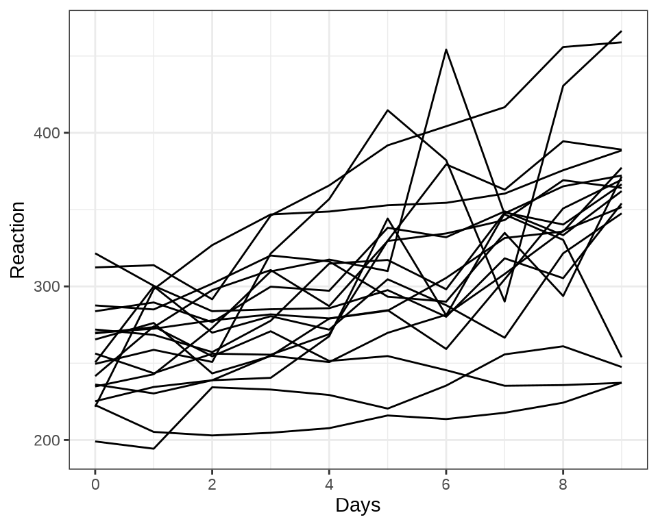
随机截距和斜率
library(nlme)
fm1 <- lme(Reaction ~ Days, random = ~ Days | Subject, data = sleepstudy)
summary(fm1)
#> Linear mixed-effects model fit by REML
#> Data: sleepstudy
#> AIC BIC logLik
#> 1755.628 1774.719 -871.8141
#>
#> Random effects:
#> Formula: ~Days | Subject
#> Structure: General positive-definite, Log-Cholesky parametrization
#> StdDev Corr
#> (Intercept) 24.740241 (Intr)
#> Days 5.922103 0.066
#> Residual 25.591843
#>
#> Fixed effects: Reaction ~ Days
#> Value Std.Error DF t-value p-value
#> (Intercept) 251.40510 6.824516 161 36.83853 0
#> Days 10.46729 1.545783 161 6.77151 0
#> Correlation:
#> (Intr)
#> Days -0.138
#>
#> Standardized Within-Group Residuals:
#> Min Q1 Med Q3 Max
#> -3.95355735 -0.46339976 0.02311783 0.46339621 5.17925089
#>
#> Number of Observations: 180
#> Number of Groups: 1832.1.2 贝叶斯派
32.1.2.1 cmdstanr
32.2 广义线性混合效应模型
二项分布
32.2.1 频率派
32.2.1.1 GLMMadaptive
#> 'data.frame':    56 obs. of  4 variables:
#>  $ herd     : Factor w/ 15 levels "1","2","3","4",..: 1 1 1 1 2 2 2 3 3 3 ...
#>  $ incidence: num  2 3 4 0 3 1 1 8 2 0 ...
#>  $ size     : num  14 12 9 5 22 18 21 22 16 16 ...
#> $ period : Factor w/ 4 levels "1","2","3","4": 1 2 3 4 1 2 3 1 2 3 ...library(GLMMadaptive)
fgm1 <- mixed_model(
fixed = cbind(incidence, size - incidence) ~ period,
random = ~ 1 | herd, data = cbpp, family = binomial(link = "logit")
)
summary(fgm1)#>
#> Call:
#> mixed_model(fixed = cbind(incidence, size - incidence) ~ period,
#> random = ~1 | herd, data = cbpp, family = binomial(link = "logit"))
#>
#> Data Descriptives:
#> Number of Observations: 56
#> Number of Groups: 15
#>
#> Model:
#> family: binomial
#> link: logit
#>
#> Fit statistics:
#> log.Lik AIC BIC
#> -91.98337 193.9667 197.507
#>
#> Random effects covariance matrix:
#> StdDev
#> (Intercept) 0.6475934
#>
#> Fixed effects:
#> Estimate Std.Err z-value p-value
#> (Intercept) -1.3995 0.2335 -5.9923 < 1e-04
#> period2 -0.9914 0.3068 -3.2316 0.00123091
#> period3 -1.1278 0.3268 -3.4513 0.00055793
#> period4 -1.5795 0.4276 -3.6937 0.00022101
#>
#> Integration:
#> method: adaptive Gauss-Hermite quadrature rule
#> quadrature points: 11
#>
#> Optimization:
#> method: EM
#> converged: TRUE32.2.1.2 mgcv
或使用 mgcv 包,可以得到近似的结果。随机效应部分可以看作可加的惩罚项
library(mgcv)
fgm3 <- gam(
  cbind(incidence, size - incidence) ~ period + s(herd, bs = "re"),
  data = cbpp, family = binomial(link = "logit"), method = "REML"
)
summary(fgm3)
#>
#> Family: binomial
#> Link function: logit
#>
#> Formula:
#> cbind(incidence, size - incidence) ~ period + s(herd, bs = "re")
#>
#> Parametric coefficients:
#> Estimate Std. Error z value Pr(>|z|)
#> (Intercept) -1.3670 0.2358 -5.799 6.69e-09 ***
#> period2 -0.9693 0.3040 -3.189 0.001428 **
#> period3 -1.1045 0.3241 -3.407 0.000656 ***
#> period4 -1.5519 0.4251 -3.651 0.000261 ***
#> ---
#> Signif. codes: 0 '***' 0.001 '**' 0.01 '*' 0.05 '.' 0.1 ' ' 1
#>
#> Approximate significance of smooth terms:
#> edf Ref.df Chi.sq p-value
#> s(herd) 9.66 14 32.03 3.21e-05 ***
#> ---
#> Signif. codes: 0 '***' 0.001 '**' 0.01 '*' 0.05 '.' 0.1 ' ' 1
#>
#> R-sq.(adj) = 0.515 Deviance explained = 53%
#> -REML = 93.199 Scale est. = 1 n = 56下面给出随机效应的标准差的估计及其上下限,和前面 GLMMadaptive 包和 lme4 包给出的结果也是接近的。
32.2.2 贝叶斯派
32.2.2.1 cmdstanr
32.3 非线性混合效应模型
32.3.1 频率派
32.3.1.1 nlme
Loblolly 数据集
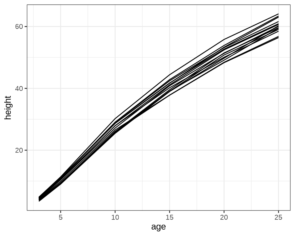
示例来自 nlme 包的函数 nlme() 帮助文档
fm1 <- nlme(height ~ SSasymp(age, Asym, R0, lrc),
  data = Loblolly,
  fixed = Asym + R0 + lrc ~ 1,
  random = Asym ~ 1,
  start = c(Asym = 103, R0 = -8.5, lrc = -3.3)
)
summary(fm1)
#> Nonlinear mixed-effects model fit by maximum likelihood
#> Model: height ~ SSasymp(age, Asym, R0, lrc)
#> Data: Loblolly
#> AIC BIC logLik
#> 239.4856 251.6397 -114.7428
#>
#> Random effects:
#> Formula: Asym ~ 1 | Seed
#> Asym Residual
#> StdDev: 3.650642 0.7188625
#>
#> Fixed effects: Asym + R0 + lrc ~ 1
#> Value Std.Error DF t-value p-value
#> Asym 101.44960 2.4616951 68 41.21128 0
#> R0 -8.62733 0.3179505 68 -27.13420 0
#> lrc -3.23375 0.0342702 68 -94.36052 0
#> Correlation:
#> Asym R0
#> R0 0.704
#> lrc -0.908 -0.827
#>
#> Standardized Within-Group Residuals:
#> Min Q1 Med Q3 Max
#> -2.23601930 -0.62380854 0.05917466 0.65727206 1.95794425
#>
#> Number of Observations: 84
#> Number of Groups: 14#> Nonlinear mixed-effects model fit by maximum likelihood
#> Model: height ~ SSasymp(age, Asym, R0, lrc)
#> Data: Loblolly
#> AIC BIC logLik
#> 238.9662 253.5511 -113.4831
#>
#> Random effects:
#> Formula: list(Asym ~ 1, lrc ~ 1)
#> Level: Seed
#> Structure: Diagonal
#> Asym lrc Residual
#> StdDev: 2.806185 0.03449969 0.6920003
#>
#> Fixed effects: Asym + R0 + lrc ~ 1
#> Value Std.Error DF t-value p-value
#> Asym 101.85205 2.3239828 68 43.82651 0
#> R0 -8.59039 0.3058441 68 -28.08747 0
#> lrc -3.24011 0.0345017 68 -93.91167 0
#> Correlation:
#> Asym R0
#> R0 0.727
#> lrc -0.902 -0.796
#>
#> Standardized Within-Group Residuals:
#> Min Q1 Med Q3 Max
#> -2.06072906 -0.69785679 0.08721706 0.73687722 1.79015782
#>
#> Number of Observations: 84
#> Number of Groups: 1432.3.2 贝叶斯派
32.3.2.1 cmdstanr
32.4 广义可加混合效应模型
从线性到可加,意味着从线性到非线性,可加模型容纳非线性的成分,比如高斯过程、样条。
32.4.1 频率派
32.4.1.1 mgcv (gam)
代码
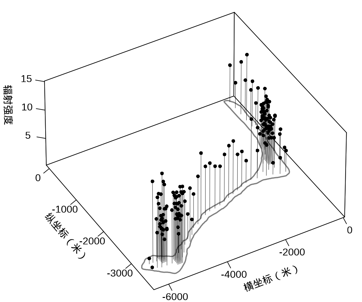
library(plot3D)
with(rongelap, {
  opar <- par(mar = c(.1, 2.5, .1, .1), no.readonly = TRUE)
  rongelap_coastline$cZ <- 0
  scatter3D(
    x = cX, y = cY, z = counts / time,
    xlim = c(-6500, 50), ylim = c(-3800, 110),
    xlab = "\n横坐标(米)", ylab = "\n纵坐标(米)",
    zlab = "\n辐射强度", lwd = 0.5, cex = 0.8,
    pch = 16, type = "h", ticktype = "detailed",
    phi = 40, theta = -30, r = 50, d = 1,
    expand = 0.5, box = TRUE, bty = "b",
    colkey = F, col = "black",
    panel.first = function(trans) {
      XY <- trans3D(
        x = rongelap_coastline$cX,
        y = rongelap_coastline$cY,
        z = rongelap_coastline$cZ,
        pmat = trans
      )
      lines(XY, col = "gray50", lwd = 2)
    }
  )
  rongelap_coastline$cZ <- NULL
  on.exit(par(opar), add = TRUE)
})
近似高斯过程、高斯过程的核函数,mgcv 包的函数 s() 帮助文档参数的说明,默认值是梅隆型相关函数及默认的范围参数,作者自己定义了一套符号约定
library(nlme)
library(mgcv)
fit_rongelap_gam <- gam(
  counts ~ s(cX, cY, bs = "gp", k = 50), offset = log(time),
  data = rongelap, family = poisson(link = "log")
)
# 模型输出
summary(fit_rongelap_gam)
#>
#> Family: poisson
#> Link function: log
#>
#> Formula:
#> counts ~ s(cX, cY, bs = "gp", k = 50)
#>
#> Parametric coefficients:
#> Estimate Std. Error z value Pr(>|z|)
#> (Intercept) 1.976815 0.001642 1204 <2e-16 ***
#> ---
#> Signif. codes: 0 '***' 0.001 '**' 0.01 '*' 0.05 '.' 0.1 ' ' 1
#>
#> Approximate significance of smooth terms:
#> edf Ref.df Chi.sq p-value
#> s(cX,cY) 48.98 49 34030 <2e-16 ***
#> ---
#> Signif. codes: 0 '***' 0.001 '**' 0.01 '*' 0.05 '.' 0.1 ' ' 1
#>
#> R-sq.(adj) = 0.876 Deviance explained = 60.7%
#> UBRE = 153.78 Scale est. = 1 n = 157#> s(cX,cY)
#> 2543.376参数 m 接受一个向量, m[1] 取值为 1 至 5,分别代表球型 spherical, 幂指数 power exponential 和梅隆型 Matern with \(\kappa\) = 1.5, 2.5 or 3.5 等 5 种相关/核函数。
#> Linking to GEOS 3.11.1, GDAL 3.6.4, PROJ 9.1.1; sf_use_s2() is TRUElibrary(abind)
library(stars)
# 类型转化
rongelap_sf <- st_as_sf(rongelap, coords = c("cX", "cY"), dim = "XY")
rongelap_coastline_sf <- st_as_sf(rongelap_coastline, coords = c("cX", "cY"), dim = "XY")
rongelap_coastline_sfp <- st_cast(st_combine(st_geometry(rongelap_coastline_sf)), "POLYGON")
# 添加缓冲区
rongelap_coastline_buffer <- st_buffer(rongelap_coastline_sfp, dist = 50)
# 构造带边界约束的网格
rongelap_coastline_grid <- st_make_grid(rongelap_coastline_buffer, n = c(150, 75))
# 将 sfc 类型转化为 sf 类型
rongelap_coastline_grid <- st_as_sf(rongelap_coastline_grid)
rongelap_coastline_buffer <- st_as_sf(rongelap_coastline_buffer)
rongelap_grid <- rongelap_coastline_grid[rongelap_coastline_buffer, op = st_intersects]
# 计算网格中心点坐标
rongelap_grid_centroid <- st_centroid(rongelap_grid)
# 共计 1612 个预测点
rongelap_grid_df <- as.data.frame(st_coordinates(rongelap_grid_centroid))
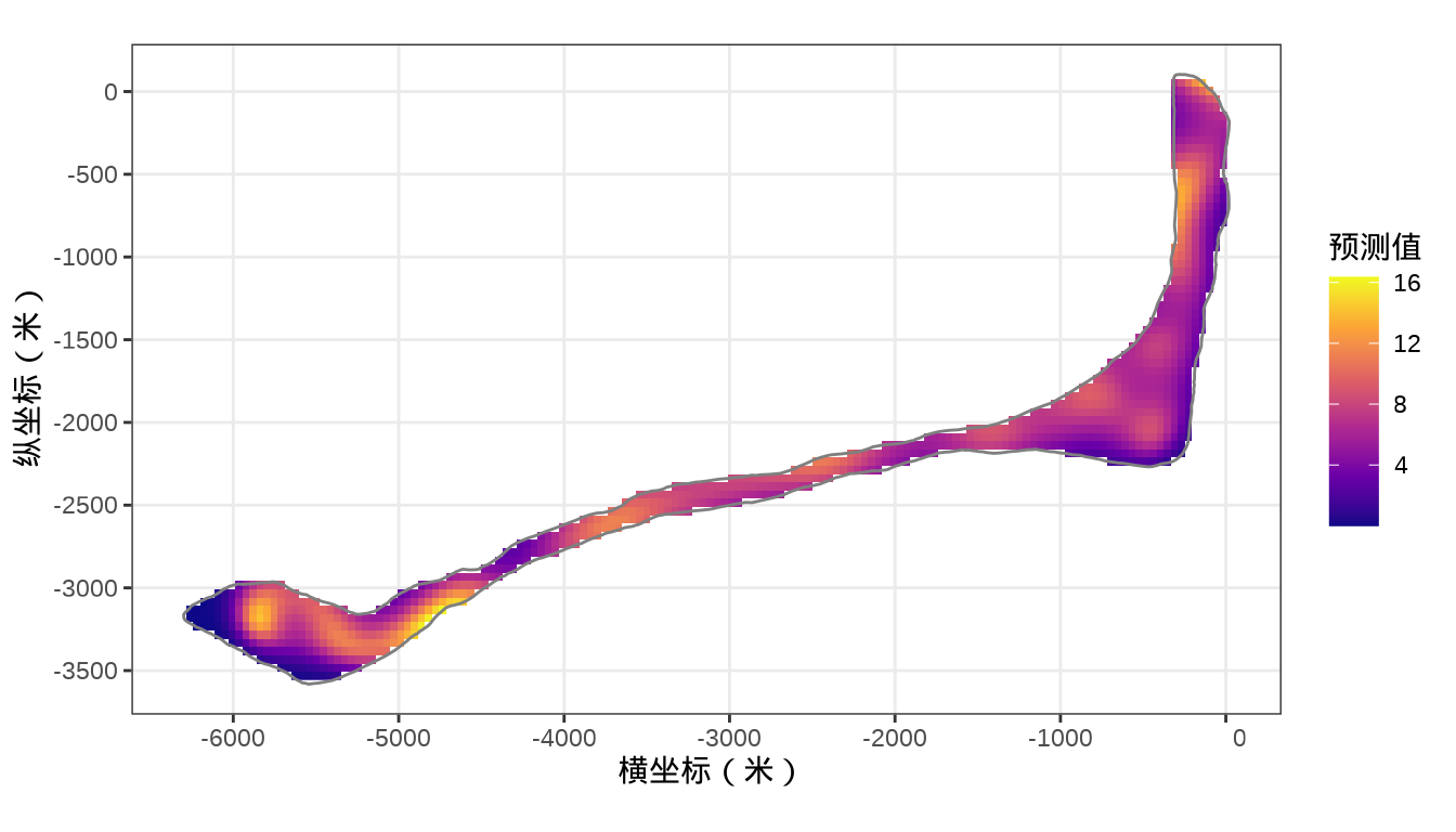
colnames(rongelap_grid_df) <- c("cX", "cY")预测和整理数据
# 预测
rongelap_grid_df$ypred <- as.vector(predict(fit_rongelap_gam, newdata = rongelap_grid_df, type = "response"))
# 整理预测数据
rongelap_grid_sf <- st_as_sf(rongelap_grid_df, coords = c("cX", "cY"), dim = "XY")
rongelap_grid_stars <- st_rasterize(rongelap_grid_sf, nx = 150, ny = 75)
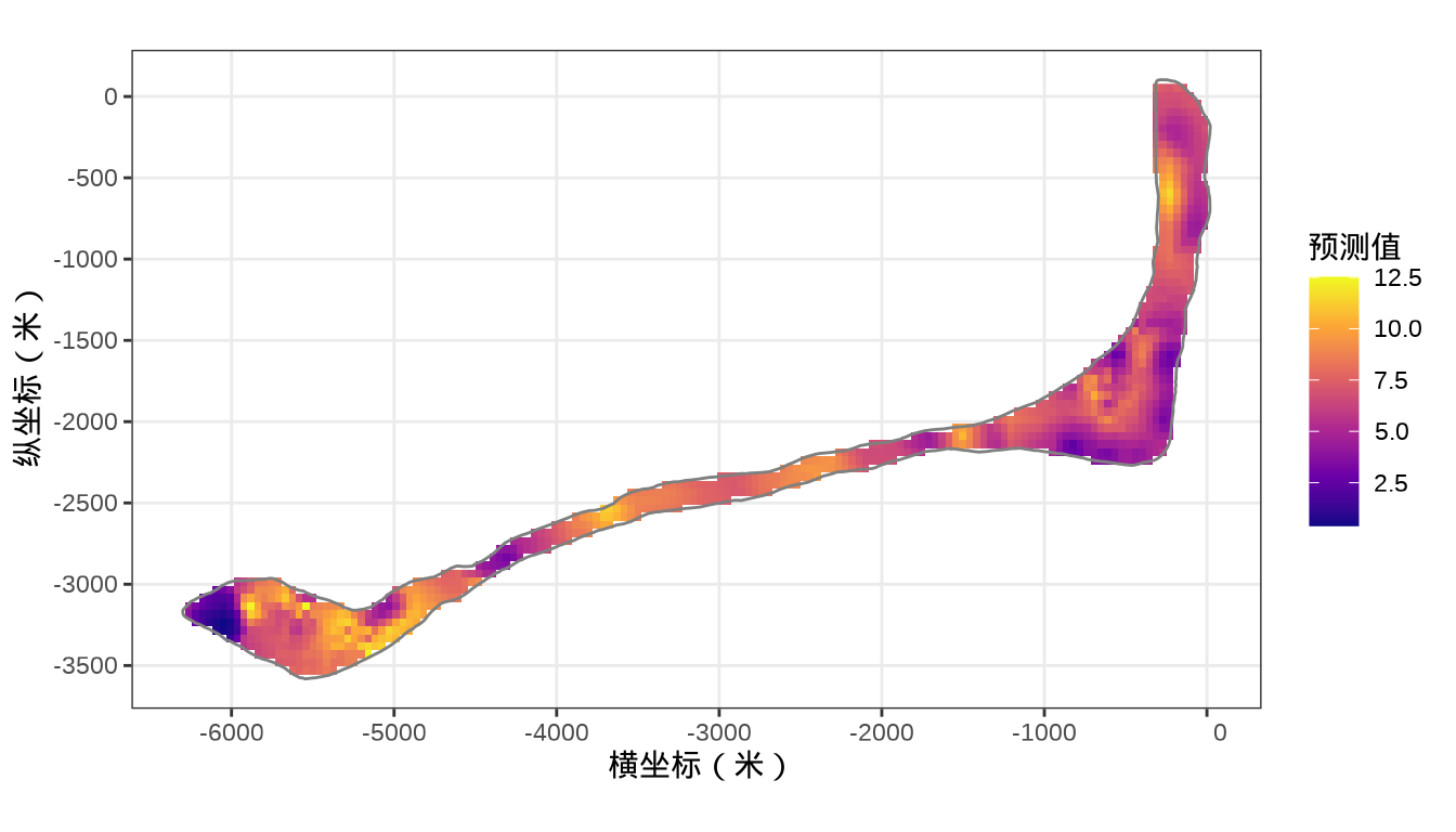
rongelap_stars <- st_crop(x = rongelap_grid_stars, y = rongelap_coastline_sfp)核辐射强度的空间分布
代码
32.4.1.2 mgcv (ginla)
mgcv 包的函数 ginla() 实现简化版 INLA
rongelap_gam <- gam(
  counts ~ s(cX, cY, bs = "gp", k = 50), offset = log(time),
  data = rongelap, family = poisson(link = "log"), fit = FALSE
)
# 简化版 INLA
fit_rongelap_ginla <- ginla(G = rongelap_gam)
str(fit_rongelap_ginla)
#> List of 2
#> $ density: num [1:50, 1:100] 2.49e-01 9.03e-06 3.51e-06 1.97e-06 1.17e-06 ...
#> $ beta : num [1:50, 1:100] 1.97 -676.61 -572.67 4720.77 240.12 ...其中, \(k = 50\) 表示 50 个参数,每个参数的分布对应有 100 个采样点,截距项的边际后验概率密度分布如下:
plot(
  fit_rongelap_ginla$beta[1, ], fit_rongelap_ginla$density[1, ],
  type = "l", xlab = "截距项", ylab = "概率密度"
)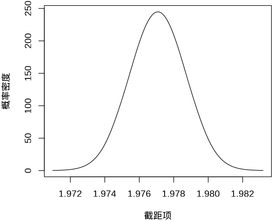
不难看出,截距项在 1.976 至 1.978 之间,各个参数的最大后验估计如下:
idx <- apply(fit_rongelap_ginla$density, 1, function(x) x == max(x))
fit_rongelap_ginla$beta[t(idx)]
#> [1] 1.977019e+00 -5.124099e+02 5.461183e+03 1.515296e+03 -2.822166e+03
#> [6] -1.598371e+04 -6.417855e+03 1.938122e+02 -4.270878e+03 3.769951e+03
#> [11] -1.002035e+04 1.914717e+03 -9.721572e+03 -3.794461e+04 -1.401549e+04
#> [16] -5.376582e+04 -1.585899e+04 -2.338235e+04 6.239053e+04 -3.574500e+02
#> [21] -4.587927e+04 1.723604e+04 -4.514781e+03 9.184026e-02 3.496526e-01
#> [26] -1.477406e+02 4.585057e+03 9.153647e+03 1.929387e+04 -1.116512e+04
#> [31] -1.166149e+04 8.079451e+02 3.627369e+03 -9.835680e+03 1.357777e+04
#> [36] 1.487742e+04 3.880562e+04 -1.708858e+03 2.775844e+04 2.527415e+04
#> [41] -3.932957e+04 3.548123e+04 -1.116341e+04 1.630910e+04 -9.789381e+02
#> [46] -2.011250e+04 2.699657e+04 -4.744393e+04 2.753347e+04 2.834356e+0432.4.2 贝叶斯派
32.4.2.1 cmdstanr
32.4.2.2 INLA
根据研究区域的边界构造非凸的内外边界,处理边界效应。
library(INLA)
library(splancs)
# 构造非凸的边界
boundary <- list(
  inla.nonconvex.hull(
    points = as.matrix(rongelap_coastline[,c("cX", "cY")]),
    convex = 100, concave = 150, resolution = 100),
  inla.nonconvex.hull(
    points = as.matrix(rongelap_coastline[,c("cX", "cY")]),
    convex = 200, concave = 200, resolution = 200)
)
根据研究区域的情况构造网格,边界内部三角网格最大边长为 300,边界外部最大边长为 600,边界外凸出距离为 100 米。
构建 SPDE,指定自协方差函数为指数型,则 \(\nu = 1/2\) ,因是二维平面,则 \(d = 2\) ,根据 \(\alpha = \nu + d/2\) ,从而 alpha = 3/2 。
生成 SPDE 模型的指标集,也是随机效应部分。
#>       s s.group  s.repl
#>     691     691     691
投影矩阵,三角网格和采样点坐标之间的投影。观测数据 rongelap 和未采样待预测的位置数据 rongelap_grid_df
# 观测位置投影到三角网格上
A <- inla.spde.make.A(mesh = mesh, loc = as.matrix(rongelap[, c("cX", "cY")]) )
# 预测位置投影到三角网格上
coop <- as.matrix(rongelap_grid_df[, c("cX", "cY")])
Ap <- inla.spde.make.A(mesh = mesh, loc = coop)
# 1612 个预测位置
dim(Ap)
#> [1] 1612 691# 在采样点的位置上估计 estimation stk.e
stk.e <- inla.stack(
tag = "est",
data = list(y = rongelap$counts, E = rongelap$time),
A = list(rep(1, 157), A),
effects = list(data.frame(b0 = 1), s = indexs)
)
# 在新生成的位置上预测 prediction stk.p
stk.p <- inla.stack(
tag = "pred",
data = list(y = NA, E = NA),
A = list(rep(1, 1612), Ap),
effects = list(data.frame(b0 = 1), s = indexs)
)
# 合并数据 stk.full has stk.e and stk.p
stk.full <- inla.stack(stk.e, stk.p)指定模型
# 模型拟合
res <- inla(formula = y ~ 0 + b0 + f(s, model = spde),
  data = inla.stack.data(stk.full),
  E = E, # E 已知漂移项
  control.family = list(link = "log"),
  control.predictor = list(
    compute = TRUE,
    link = 1, # 与 control.family 联系函数相同
    A = inla.stack.A(stk.full)
  ),
  control.compute = list(
    cpo = TRUE,
    waic = TRUE, # WAIC 统计量 通用信息准则
    dic = TRUE   # DIC 统计量 偏差信息准则
  ),
  family = "poisson"
)
# 模型输出
summary(res)
#>
#> Call:
#> c("inla.core(formula = formula, family = family, contrasts = contrasts,
#> ", " data = data, quantiles = quantiles, E = E, offset = offset, ", "
#> scale = scale, weights = weights, Ntrials = Ntrials, strata = strata,
#> ", " lp.scale = lp.scale, link.covariates = link.covariates, verbose =
#> verbose, ", " lincomb = lincomb, selection = selection, control.compute
#> = control.compute, ", " control.predictor = control.predictor,
#> control.family = control.family, ", " control.inla = control.inla,
#> control.fixed = control.fixed, ", " control.mode = control.mode,
#> control.expert = control.expert, ", " control.hazard = control.hazard,
#> control.lincomb = control.lincomb, ", " control.update =
#> control.update, control.lp.scale = control.lp.scale, ", "
#> control.pardiso = control.pardiso, only.hyperparam = only.hyperparam,
#> ", " inla.call = inla.call, inla.arg = inla.arg, num.threads =
#> num.threads, ", " keep = keep, working.directory = working.directory,
#> silent = silent, ", " inla.mode = inla.mode, safe = FALSE, debug =
#> debug, .parent.frame = .parent.frame)" )
#> Time used:
#> Pre = 1.35, Running = 2.92, Post = 0.123, Total = 4.39
#> Fixed effects:
#> mean sd 0.025quant 0.5quant 0.975quant mode kld
#> b0 1.828 0.061 1.706 1.828 1.948 1.828 0
#>
#> Random effects:
#> Name Model
#> s SPDE2 model
#>
#> Model hyperparameters:
#> mean sd 0.025quant 0.5quant 0.975quant mode
#> Theta1 for s 2.00 0.062 1.88 2.00 2.12 2.00
#> Theta2 for s -4.85 0.129 -5.11 -4.85 -4.60 -4.85
#>
#> Deviance Information Criterion (DIC) ...............: 1834.57
#> Deviance Information Criterion (DIC, saturated) ....: 314.90
#> Effective number of parameters .....................: 156.46
#>
#> Watanabe-Akaike information criterion (WAIC) ...: 1789.31
#> Effective number of parameters .................: 80.06
#>
#> Marginal log-Likelihood: -1331.95
#> CPO, PIT is computed
#> Posterior summaries for the linear predictor and the fitted values are computed
#> (Posterior marginals needs also 'control.compute=list(return.marginals.predictor=TRUE)')kld 表示 Kullback-Leibler divergence (KLD) 它的值描述标准高斯分布与 Simplified Laplace Approximation 之间的差别,值越小越表示拉普拉斯的近似效果好。
DIC 和 WAIC 指标都是评估模型预测表现的。另外,还有两个量计算出来了,但是没有显示,分别是 CPO 和 PIT 。CPO 表示 Conditional Predictive Ordinate (CPO),PIT 表示 Probability Integral Transforms (PIT) 。
固定效应和超参数部分
#>        mean         sd 0.025quant 0.5quant 0.975quant     mode          kld
#> b0 1.828055 0.06149404 1.706407 1.828313 1.948236 1.828308 1.787791e-08#> mean sd 0.025quant 0.5quant 0.975quant mode
#> Theta1 for s 2.000472 0.0623746 1.876914 2.000733 2.122506 2.001822
#> Theta2 for s -4.851586 0.1289191 -5.104743 -4.851809 -4.597131 -4.852738预测数据
# 预测值对应的指标集合
index <- inla.stack.index(stk.full, tag = "pred")$data
# 提取预测结果,后验均值
# pred_mean <- res$summary.fitted.values[index, "mean"]
# 95% 预测下限
# pred_ll <- res$summary.fitted.values[index, "0.025quant"]
# 95% 预测上限
# pred_ul <- res$summary.fitted.values[index, "0.975quant"]
# 整理数据
rongelap_grid_df$ypred <- res$summary.fitted.values[index, "mean"]
# 预测值数据
rongelap_grid_sf <- st_as_sf(rongelap_grid_df, coords = c("cX", "cY"), dim = "XY")
rongelap_grid_stars <- st_rasterize(rongelap_grid_sf, nx = 150, ny = 75)
rongelap_stars <- st_crop(x = rongelap_grid_stars, y = rongelap_coastline_sfp)
预测结果
32.5 总结
通过对频率派和贝叶斯派方法的比较,发现一些有意思的结果。与 Stan 不同,INLA 包做近似贝叶斯推断,计算效率很高。
集成嵌套拉普拉斯近似 (Integrated Nested Laplace Approximations,简称 INLA),INLA 软件能处理上千个高斯随机效应,但最多只能处理 15 个超参数,因为 INLA 使用 CCD 处理超参数,如果使用 MCMC 处理超参数,就有可能处理更多的超参数,如 GPstuff 使用 MCMC 而不是 CCD 处理超参数,Daniel Simpson 等把 Laplace approximation 带入 Stan,这样就可以处理上千个超参数。 更多内容见 2009 年 INLA 诞生的论文和《Advanced Spatial Modeling with Stochastic Partial Differential Equations Using R and INLA》中估计方法章节 CCD。
32.6 习题
基于奥克兰火山地形数据集 volcano ,随机拆分成训练数据和测试数据,训练数据可以看作采样点的观测数据,建立高斯过程回归模型,比较测试数据与未采样的位置上的预测数据,在计算速度、准确度、易用性等方面总结 Stan 和 INLA 的特点。
-
基于 MASS 包的地形数据集 topo,建立高斯过程回归模型,比较贝叶斯预测与克里金插值预测的效果。
代码
data(topo, package = "MASS") set.seed(20232023) nchains <- 2 # 2 条迭代链 # 给每条链设置不同的参数初始值 inits_data_gaussian <- lapply(1:nchains, function(i) { list( beta = rnorm(1), sigma = runif(1), phi = runif(1), tau = runif(1) ) }) # 预测区域网格化 nx <- ny <- 27 topo_grid_df <- expand.grid( x = seq(from = 0, to = 6.5, length.out = nx), y = seq(from = 0, to = 6.5, length.out = ny) ) # 对数高斯模型 topo_gaussian_d <- list( N1 = nrow(topo), # 观测记录的条数 N2 = nrow(topo_grid_df), D = 2, # 2 维坐标 x1 = topo[, c("x", "y")], # N x 2 坐标矩阵 x2 = topo_grid_df[, c("x", "y")], y1 = topo[, "z"] # N 向量 ) library(cmdstanr) # 编码 mod_topo_gaussian <- cmdstan_model( stan_file = "code/gaussian_process_pred.stan", compile = TRUE, cpp_options = list(stan_threads = TRUE) ) # 高斯过程回归模型 fit_topo_gaussian <- mod_topo_gaussian$sample( data = topo_gaussian_d, # 观测数据 init = inits_data_gaussian, # 迭代初值 iter_warmup = 500, # 每条链预处理迭代次数 iter_sampling = 1000, # 每条链总迭代次数 chains = nchains, # 马尔科夫链的数目 parallel_chains = 2, # 指定 CPU 核心数,可以给每条链分配一个 threads_per_chain = 1, # 每条链设置一个线程 show_messages = FALSE, # 不显示迭代的中间过程 refresh = 0, # 不显示采样的进度 output_dir = "data-raw/", seed = 20232023 ) # 诊断 fit_topo_gaussian$diagnostic_summary() # 对数高斯模型 fit_topo_gaussian$summary( variables = c("lp__", "beta", "sigma", "phi", "tau"), .num_args = list(sigfig = 4, notation = "dec") ) # 未采样的位置的预测值 ypred <- fit_topo_gaussian$summary(variables = "ypred", "mean") # 预测值 topo_grid_df$ypred <- ypred$mean # 整理数据 library(sf) topo_grid_sf <- st_as_sf(topo_grid_df, coords = c("x", "y"), dim = "XY") library(stars) # 26x26 的网格 topo_grid_stars <- st_rasterize(topo_grid_sf, nx = 26, ny = 26) library(ggplot2) ggplot() + geom_stars(data = topo_grid_stars, aes(fill = ypred)) + scale_fill_viridis_c(option = "C") + theme_bw() -
用 brms 包实现贝叶斯高斯过程回归模型,考虑用样条近似高斯过程以加快计算。提示:brms 包的函数
gp()的参数 \(k\) 表示近似高斯过程 GP 所用的基函数的数目。截止写作时间,函数gp()的参数cov只能取指数二次核函数 exponentiated-quadratic kernel 。代码
# 高斯过程近似计算
bgamm2 <- brms::brm(
  z ~ gp(x, y, cov = "exp_quad", c = 5 / 4, k = 50),
  data = topo, chains = 2, seed = 20232023,
  warmup = 1000, iter = 2000, thin = 1, refresh = 0,
  control = list(adapt_delta = 0.99)
)
# 输出结果
summary(bgamm2)
# 条件效应
me3 <- brms::conditional_effects(bgamm1, ndraws = 200, spaghetti = TRUE)
# 绘制图形
plot(me3, ask = FALSE, points = TRUE)